
Line of Best Fit and R²: Choosing the Right Trend Line
By Dr. Ahmed Mortuza Saleque · Updated · How we check our content
The short answer
A line of best fit is the line that makes the squared vertical distances from the points as small as possible. R squared (R²) is the share of the variation in y that the line explains, from 0 to 1. In the example below, y = 4.48x + 46.9 has R² = 0.99. Pick the fit type that matches the shape of the data, not the highest R² alone.
Open the Data Plotter →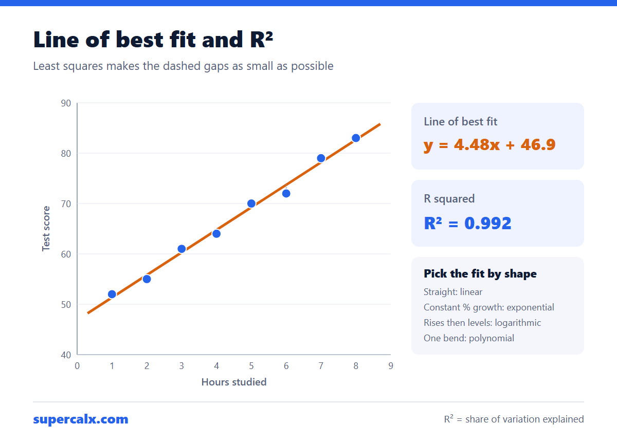
Worked example: the data
Eight students: hours of study and test score.
| Hours studied (x) | Test score (y) |
|---|---|
| 1 | 52 |
| 2 | 55 |
| 3 | 61 |
| 4 | 64 |
| 5 | 70 |
| 6 | 72 |
| 7 | 79 |
| 8 | 83 |
Calculating the line of best fit
- Means: x̄ = 4.5 and ȳ = 67.0.
- Slope = Σ(x − x̄)(y − ȳ) ÷ Σ(x − x̄)² = 188 ÷ 42 = 4.48 points per hour.
- Intercept = ȳ − slope × x̄ = 67.0 − 4.48 × 4.5 = 46.9.
- Line of best fit: score = 4.48 × hours + 46.9.
- R² = 0.992: the line explains 99.2% of the variation in scores.
Paste the two columns into the Data Plotter and choose Linear regression to get the same equation and R² drawn on the chart.
What R² does and does not tell you
- R² does not prove cause. Ice cream sales and drownings correlate because both rise in summer.
- A high R² can hide the wrong shape. Always look at the residual plot: a curve in the residuals means the model is wrong.
- Adding polynomial terms always raises R², even when the extra wiggles are noise.
- For a straight line, R² is the square of the correlation coefficient r. The correlation coefficient calculator gives r directly.
The Data Plotter labels fits with these bands.
| R² | Label | Meaning |
|---|---|---|
| Above 0.9 | Excellent | The fit follows the data closely |
| 0.7 to 0.9 | Good | Clear trend with some scatter |
| 0.5 to 0.7 | Moderate | A trend, but much is unexplained |
| Below 0.5 | Weak | The model explains little |
Choosing the fit type
| Fit | Equation | Use when | Requirement |
|---|---|---|---|
| Linear | y = a + bx | Constant rate of change | None |
| Exponential | y = a·e^(bx) | Growth or decay by a constant percentage | y > 0 |
| Logarithmic | y = a + b·ln(x) | Fast rise that levels off | x > 0 |
| Power | y = a·x^b | Scaling laws, such as area and length | x and y > 0 |
| Polynomial | y = a + bx + cx² … | One or two bends, within the data range | Use the lowest degree that works |
Example: when linear is the wrong choice
A bacterial culture is counted every hour: 100, 135, 180, 245, 330, 445 and 600. A straight line gives R² = 0.94, which sounds good, but its residuals curve. An exponential fit, y = 99.8·e^(0.299x), gives R² above 0.999 and matches the biology: the count grows about 35% an hour and doubles every ln 2 ÷ 0.299 = 2.3 hours.
The Data Plotter's Model Comparison chart fits linear, polynomial, exponential, logarithmic and power models at once and ranks them by R², so you can see this in one click.
Common questions
How do you find the line of best fit?
Use least squares: slope = Σ(x − x̄)(y − ȳ) ÷ Σ(x − x̄)², intercept = ȳ − slope × x̄. A plotting tool does this automatically.
What is a good R squared value?
It depends on the field. Physical experiments often exceed 0.95; social and biological data with R² of 0.3 to 0.6 can still be useful.
Can R squared be negative?
For a least-squares fit with an intercept, no. It can be negative when a model is forced through a point or judged on new data, meaning it predicts worse than the mean.
Should I extrapolate the line beyond my data?
Carefully. The fit is only checked within the data range; predictions far outside it, such as 20 hours of study, can be unrealistic.
Calculators for this article
More from the blog
 Gantt Chart for a Research Proposal: Example and Template
 PhD and Thesis Gantt Chart: Timeline Example by Month
 Gantt Chart Milestones and Deliverables: How to Show Them
 Gantt Chart vs PERT Chart vs Timeline: Which to Use
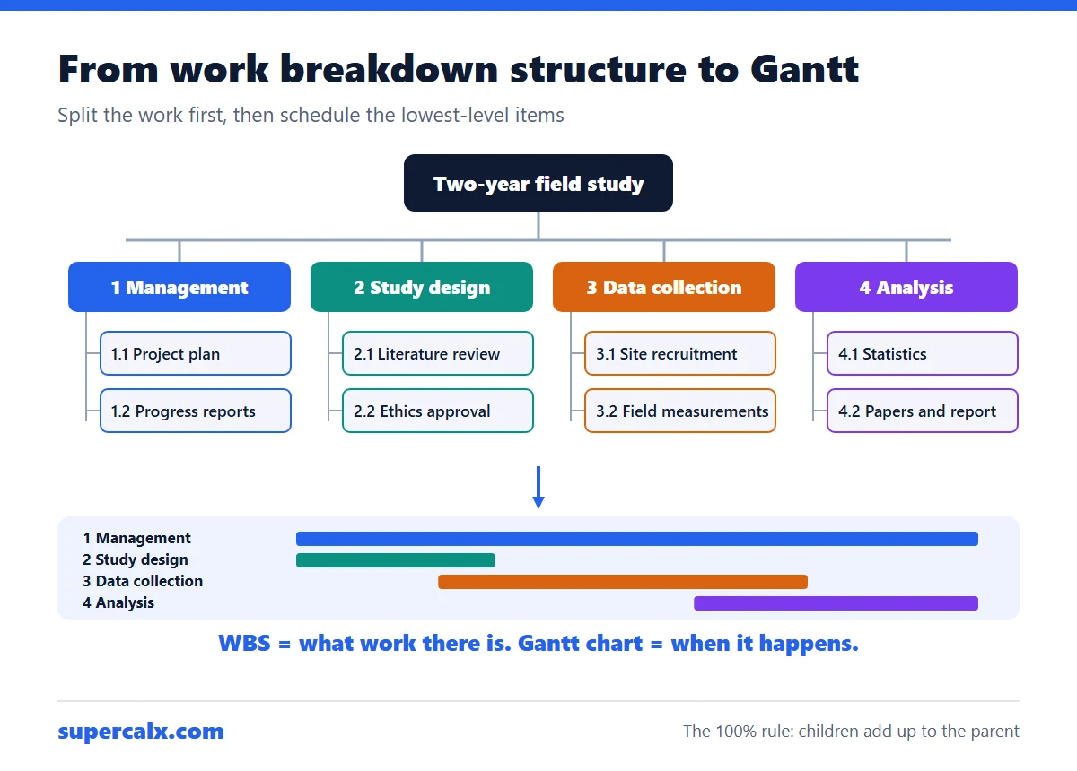 Work Breakdown Structure Example: From WBS to Gantt Chart
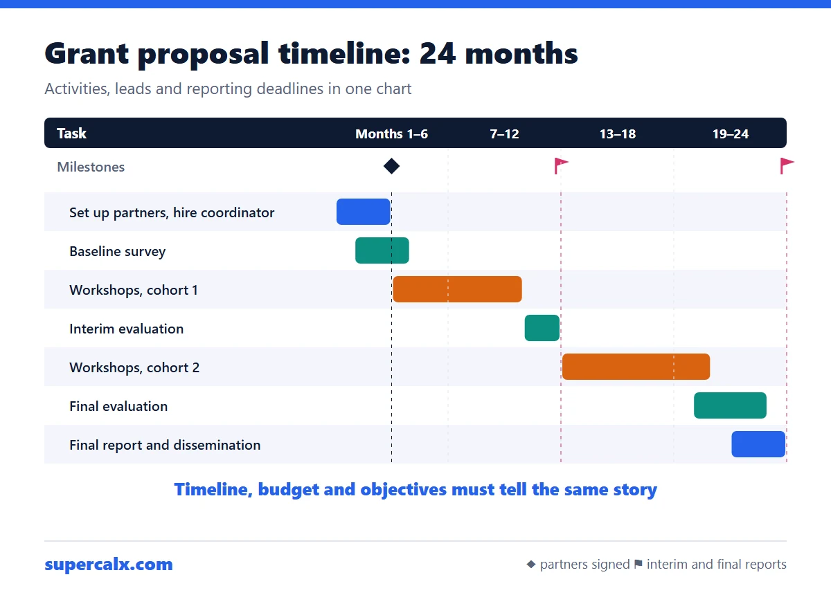 How to Write a Grant Proposal Timeline (With Example)
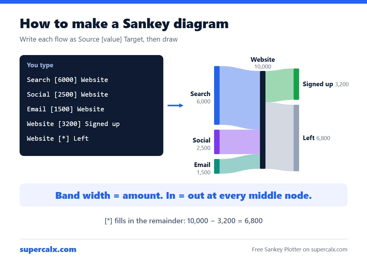 How to Make a Sankey Diagram (Free, No Excel Add-in)
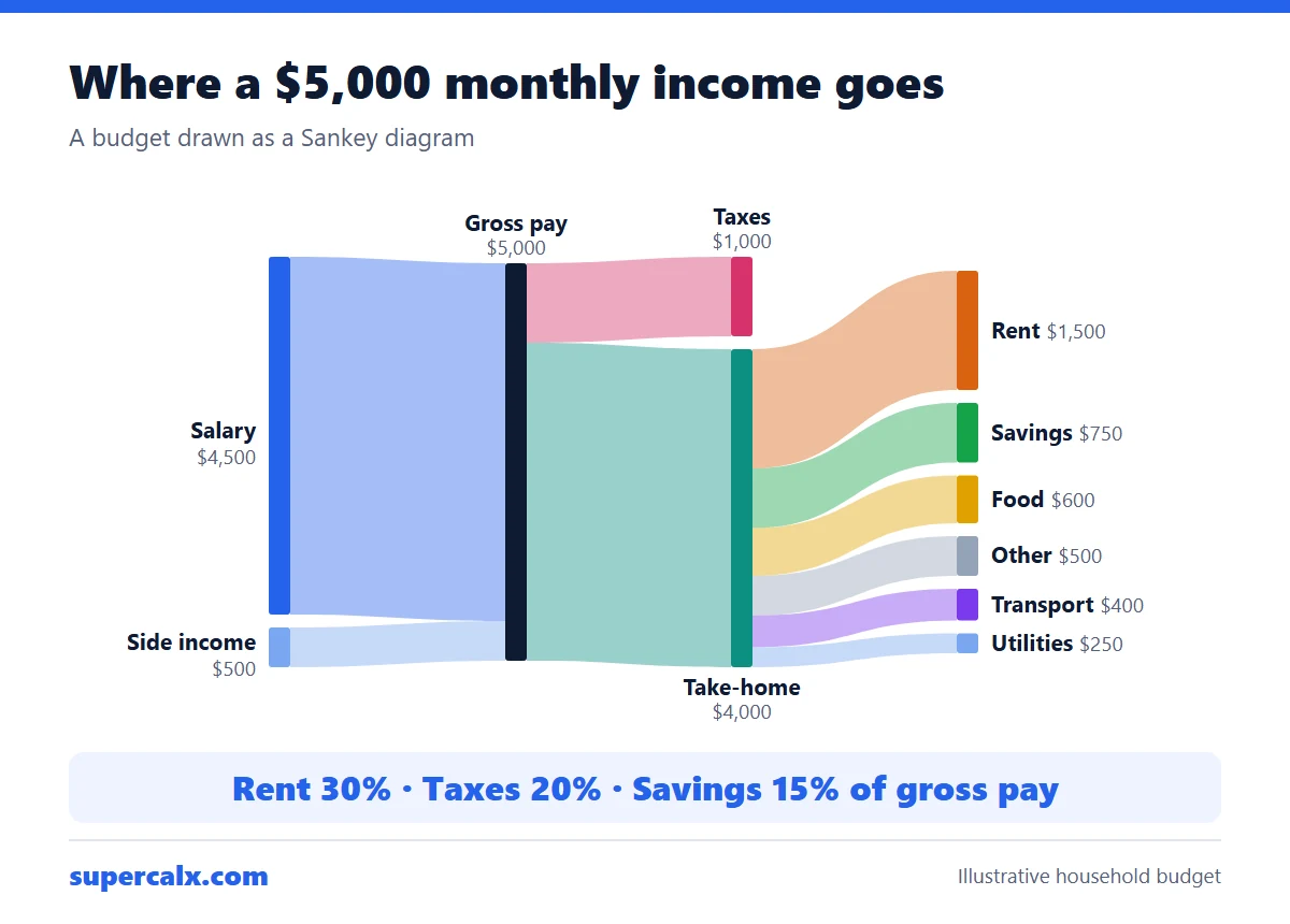 Sankey Diagram for a Budget: See Where Your Money Goes